Clustergram

Visualization and diagnostics for cluster analysis

Clustergram is a diagram proposed by Matthias Schonlau in his paper The clustergram: A graph for visualizing hierarchical and nonhierarchical cluster analyses:

In hierarchical cluster analysis, dendrograms are used to visualize how clusters are formed. I propose an alternative graph called a “clustergram” to examine how cluster members are assigned to clusters as the number of clusters increases. This graph is useful in exploratory analysis for nonhierarchical clustering algorithms such as k-means and for hierarchical cluster algorithms when the number of observations is large enough to make dendrograms impractical.

The clustergram was later implemented in R by Tal Galili, who also gives a thorough explanation of the concept.

This is a Python implementation, originally based on Tal's script, written for scikit-learn and RAPIDS cuML implementations of K-Means, Mini Batch K-Means and Gaussian Mixture Model (scikit-learn only) clustering, plus hierarchical/agglomerative clustering using SciPy. Alternatively, you can create clustergram using from_* constructors based on alternative clustering algorithms.

Getting started

You can install clustergram from conda or pip:

conda install clustergram -c conda-forge

pip install clustergram

In any case, you still need to install your selected backend (scikit-learn and scipy or cuML).

The example of clustergram on Palmer penguins dataset:

import seaborn
df = seaborn.load_dataset('penguins')

First we have to select numerical data and scale them.

from sklearn.preprocessing import scale
data = scale(df.drop(columns=['species', 'island', 'sex']).dropna())

And then we can simply pass the data to clustergram.

from clustergram import Clustergram

cgram = Clustergram(range(1, 8))
cgram.fit(data)
cgram.plot()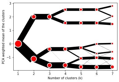

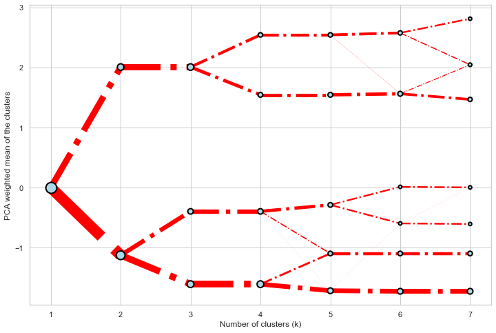
Styling

Clustergram.plot() returns matplotlib axis and can be fully customised as any other matplotlib plot.

seaborn.set(style='whitegrid')

cgram.plot(
    ax=ax,
    size=0.5,
    linewidth=0.5,
    cluster_style={"color": "lightblue", "edgecolor": "black"},
    line_style={"color": "red", "linestyle": "-."},
    figsize=(12, 8)
)

Mean options

On the y axis, a clustergram can use mean values as in the original paper by Matthias Schonlau or PCA weighted mean values as in the implementation by Tal Galili.

cgram = Clustergram(range(1, 8))
cgram.fit(data)
cgram.plot(figsize=(12, 8), pca_weighted=True)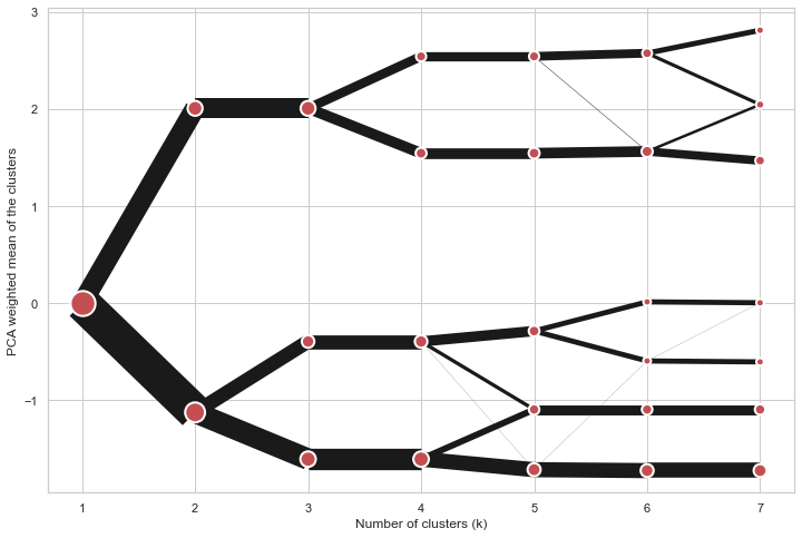

cgram = Clustergram(range(1, 8))
cgram.fit(data)
cgram.plot(figsize=(12, 8), pca_weighted=False)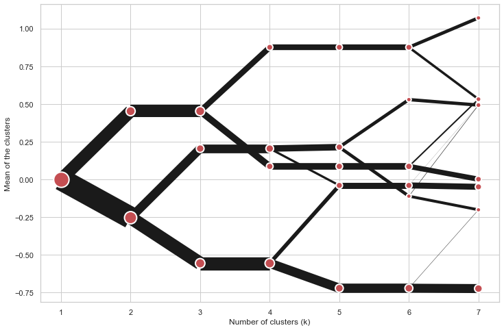

Scikit-learn, SciPy and RAPIDS cuML backends

Clustergram offers three backends for the computation - scikit-learn and scipy which use CPU and RAPIDS.AI cuML, which uses GPU. Note that all are optional dependencies but you will need at least one of them to generate clustergram.

Using scikit-learn (default):

cgram = Clustergram(range(1, 8), backend='sklearn')
cgram.fit(data)
cgram.plot()

Using cuML:

cgram = Clustergram(range(1, 8), backend='cuML')
cgram.fit(data)
cgram.plot()

data can be all data types supported by the selected backend (including cudf.DataFrame with cuML backend).

Supported methods

Clustergram currently supports K-Means, Mini Batch K-Means, Gaussian Mixture Model and SciPy's hierarchical clustering methods. Note tha GMM and Mini Batch K-Means are supported only for scikit-learn backend and hierarchical methods are supported only for scipy backend.

Using K-Means (default):

cgram = Clustergram(range(1, 8), method='kmeans')
cgram.fit(data)
cgram.plot()

Using Mini Batch K-Means, which can provide significant speedup over K-Means:

cgram = Clustergram(range(1, 8), method='minibatchkmeans', batch_size=100)
cgram.fit(data)
cgram.plot()

Using Gaussian Mixture Model:

cgram = Clustergram(range(1, 8), method='gmm')
cgram.fit(data)
cgram.plot()

Using Ward's hierarchical clustering:

cgram = Clustergram(range(1, 8), method='hierarchical', linkage='ward')
cgram.fit(data)
cgram.plot()

Manual input

Alternatively, you can create clustergram using from_data or from_centers methods based on alternative clustering algorithms.

Using Clustergram.from_data which creates cluster centers as mean or median values:

data = numpy.array([[-1, -1, 0, 10], [1, 1, 10, 2], [0, 0, 20, 4]])
labels = pandas.DataFrame({1: [0, 0, 0], 2: [0, 0, 1], 3: [0, 2, 1]})

cgram = Clustergram.from_data(data, labels)
cgram.plot()

Using Clustergram.from_centers based on explicit cluster centers.:

labels = pandas.DataFrame({1: [0, 0, 0], 2: [0, 0, 1], 3: [0, 2, 1]})
centers = {
            1: np.array([[0, 0]]),
            2: np.array([[-1, -1], [1, 1]]),
            3: np.array([[-1, -1], [1, 1], [0, 0]]),
        }
cgram = Clustergram.from_centers(centers, labels)
cgram.plot(pca_weighted=False)

To support PCA weighted plots you also need to pass data:

cgram = Clustergram.from_centers(centers, labels, data=data)
cgram.plot()

Partial plot

Clustergram.plot() can also plot only a part of the diagram, if you want to focus on a limited range of k.

cgram = Clustergram(range(1, 20))
cgram.fit(data)
cgram.plot(figsize=(12, 8))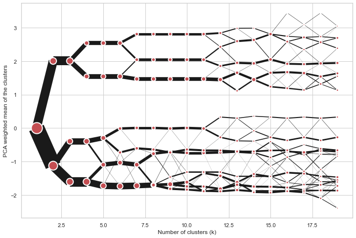

cgram.plot(k_range=range(3, 10), figsize=(12, 8))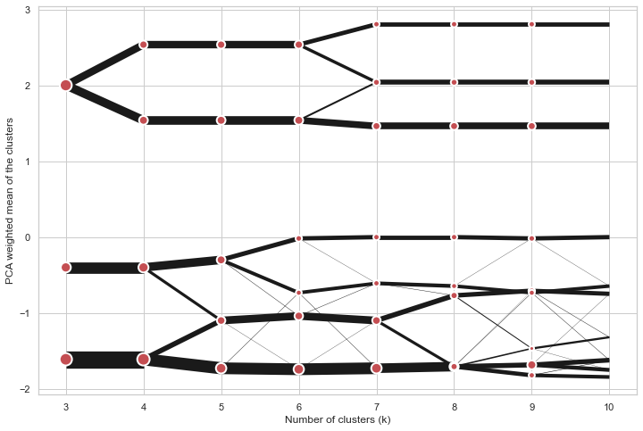

Additional clustering performance evaluation

Clustergam includes handy wrappers around a selection of clustering performance metrics offered by scikit-learn. Data which were originally computed on GPU are converted to numpy on the fly.

Silhouette score

Compute the mean Silhouette Coefficient of all samples. See scikit-learn documentation for details.

>>> cgram.silhouette_score()
2    0.531540
3    0.447219
4    0.400154
5    0.377720
6    0.372128
7    0.331575
Name: silhouette_score, dtype: float64

Once computed, the resulting Series is available as cgram.silhouette_. Calling the original method will recompute the score.

Calinski and Harabasz score

Compute the Calinski and Harabasz score, also known as the Variance Ratio Criterion. See scikit-learn documentation for details.

>>> cgram.calinski_harabasz_score()
2    482.191469
3    441.677075
4    400.392131
5    411.175066
6    382.731416
7    352.447569
Name: calinski_harabasz_score, dtype: float64

Once computed, the resulting Series is available as cgram.calinski_harabasz_. Calling the original method will recompute the score.

Davies-Bouldin score

Compute the Davies-Bouldin score. See scikit-learn documentation for details.

>>> cgram.davies_bouldin_score()
2    0.714064
3    0.943553
4    0.943320
5    0.973248
6    0.950910
7    1.074937
Name: davies_bouldin_score, dtype: float64

Once computed, the resulting Series is available as cgram.davies_bouldin_. Calling the original method will recompute the score.

Accessing labels

Clustergram stores resulting labels for each of the tested options, which can be accessed as:

>>> cgram.labels_
     1  2  3  4  5  6  7
0    0  0  2  2  3  2  1
1    0  0  2  2  3  2  1
2    0  0  2  2  3  2  1
3    0  0  2  2  3  2  1
4    0  0  2  2  0  0  3
..  .. .. .. .. .. .. ..
337  0  1  1  3  2  5  0
338  0  1  1  3  2  5  0
339  0  1  1  1  1  1  4
340  0  1  1  3  2  5  5
341  0  1  1  1  1  1  5

Saving clustergram

You can save both the plot and clustergram.Clustergram to a disk.

Saving plot

Clustergram.plot() returns matplotlib axis object and as such can be saved as any other plot:

import matplotlib.pyplot as plt

cgram.plot()
plt.savefig('clustergram.svg')

Saving object

If you want to save your computed clustergram.Clustergram object to a disk, you can use pickle library:

import pickle

with open('clustergram.pickle','wb') as f:
    pickle.dump(cgram, f)

Then loading is equally simple:

with open('clustergram.pickle','rb') as f:
    loaded = pickle.load(f)

References

Schonlau M. The clustergram: a graph for visualizing hierarchical and non-hierarchical cluster analyses. The Stata Journal, 2002; 2 (4):391-402.

Schonlau M. Visualizing Hierarchical and Non-Hierarchical Cluster Analyses with Clustergrams. Computational Statistics: 2004; 19(1):95-111.

https://www.r-statistics.com/2010/06/clustergram-visualization-and-diagnostics-for-cluster-analysis-r-code/