Dynamical-Systems-Basics

Preamble

This write up is based on material from Steve Brunton's amazing course on youtube Differential Equations and Dynamical Systems. If you haven't seen this series, definitely go check it out, it gives you an intuitive sense for why you should care about dynamical systems, some practical examples and how to solve them.

I'm writing this is part because I forget things that I've learned easily and so this is just a means by which I'm hoping to both give myself a refresher and a resource to come back to later.

All the code for the graphs will be organized in intuitive subfolders. I'm running python 3.8 with numpy, scipy, and matplotlib installed.

Motivation

So why should you care about dynamical systems? What a great question! Dynamical systems are all around us, you can see them in action in simple objects and phenomena in your everyday life. The motion of the bobble head on your desk? Dynamical system. The number of cases of Covid19? Dynamical system. The fuel consumption of your car? Dynamical system. Everytime, the rate of change of a variable in time is related to the quantity of the variable at that time you have a dynamical system. These systems give us a new tool for us to place in our modeling toolkits. Alright, lets get our hands dirty.

First Order Linear Differential Equations

$\frac{d}{dt}x(t) = \lambda x(t)$

Wow, what a mouthful of a subtitle. Lets break it down with the example above. The First Order part comes from the fact that for the variable that we are concerned with $x(t)$, we only use its first derivative in the equation. The Linear part comes from the fact that the expression on the right hand side is a linear function of our variable $x(t)$. And of course, because our equation involves the derivative of our variable we have the term Differential Equation being used. This type of equation is part of a more general class of equations call Ordinary Differential Equations or ODEs for short. We say Ordinary because we only use the normal derivatives in our equations and not the partial derivatives.

As an aside, lets take a look at some simplified notation. The first thing we're going to do is drop the $(t)$ evaluations. We're going to assume that they're still there, but we'll only use that notation when we're actually evaluating them at some value $t=a$.

$\frac{d}{dt}x = \lambda x$

Alright, the last thing we'll do is drop represent $\frac{dx}{dt}$ by $\dot{x}$. If you see double dot notation that just means the second derivative and so on for higher order derivatives. So finally we have:

$\dot{x} = \lambda x$

Lets try to come up with a solution for this equation. But what do we even mean by a solution? Basically we're just trying to figure out what this equation tells us about our variable $x(t)$ as it evolves in time. We are looking for a relation between the dependent variable $x(t)$ and the independent variable $t$ in the form of an equation.

Okay, so at first glance it might look like our equation above doesn't really tell us anything about the variable $x(t)$ in time. This sort of looks like a chicken or the egg scenario. How do we compute the derivative of our variable $x(t)$ if we first need the derivative to define the variable? Kinda odd isn't it?

We have a few options here. We can either try to solve these types of equations by simply manipulating the variables we have, or we can try to approximate the solution the first method might give us. First, we're going investigate the method of manipulating the variables we have; this is what we call an Analytic Solution.

Analytic Solutions

There are many ways to come up with an analytic solution. Let's look at one for now, and we'll look at three more methods later.

Method 1: Magic (Sort of)

$\dot{x} = \lambda x, \lambda \in \mathbb{R}$

Let's look at our motivating example first. As we mentioned before this one is a first order ODE. The first thing we ask ourselves is "what functions do I know who's derivative is just a constant times itself." Well, we don't even really need an exact solution at this point, we just need some functions that sort of behave this way. A couple of function classes in our toolkit exhibit this cyclical behaviour when being differentiated. We have functions like $e^t$, $sin(t)$ and $cos(t)$.

For $e^t$ we know it's derivative is equal to itself.

$\frac{d}{dt} e^t = e^t$

This seems like the function we want to be using with the addition that we'll make use of the chain rule. To understand why we won't use $sin(t)$ or $cos(t)$ in this particular situation differentiate $sin(t)$ and notice that no matter the choice for the constant $\lambda$ our differential equation doesn't hold since $\lambda$ only scales $sin(t)$'s amplitude.

Ok so lets play around with $e^t$. Let's say we choose $x(t) = e^t$ as our guess at the solution. If we take its derivative, we end up with the same function. Looking at our differential equation, we are still missing a constant factor of $\lambda$ for the derivative.

$\frac{d}{dt} e^t = e^t$

Let's take a look at how this function's derivative behaves when we modify the exponent. If we add a factor $\lambda$ infront of $t$ we get the following derivative:

$\frac{d}{dt} e^{\lambda t} = \lambda e^{\lambda t}$

Take a hard look, do you see anything interesting? Yup! Its our solution. We take $x(t) = e^{\lambda t}$. Now if we substitute in our function $x(t)$ we have:

$\frac{d}{dt} e^{\lambda t} = \frac{d}{dt} x(t) = \lambda x(t) \rightarrow{} \dot{x} = \lambda x$

If you feel like what you just watched was magic trick then you'd sort of be correct. All that we did is basically just guessed a solution that happened to work for this particular ODE.

There's one thing that we forgot to talk about. If you take a look at our solution, there's one thing missing. If we would have choosen $x(t) = ce^{\lambda t}, c \in \mathbb{R}$ to be our guess, we would have gotten another solution. Go on, try it out on paper!

That's interesting, so it seems that for any constant $c \in \mathbb{R}$ we have a solution. You might ask, what exactly this constant $c$ represent. Let's think of this differential equation as a model for a particle at time $t$. Below, I'm going to show you a graph of our original solution with $c = 1$.

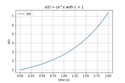
If you look closely, you'll notice that at time $t = 0$, $x(t) = 1$. When we plug in $t = 0$ into our more general solution it simplifies to $x(0) = c$. We can come to the conclusion that $c$ is the initial condition of our general system. We will denote this by $x_0$.

This leads us to the general class of solutions to our problem:

$x(t) = e^{\lambda t} x_0$

Method 2: Taylor Series

Let's take a look at this from a bit of a different perspective. We're going to try to harness power of Taylor series to help us come up with a solution to our differential equation. For those, who haven't seen Taylor series before, I'll give you a brief introduction.

For functions that are continuous and infinitely differentiable, we can come up with an exact representations just using an infinite sum of polynomial terms, centering our approximation around a point $c$. We can represent functions like $e^t$, $sin(t)$ and $cos(t)$ like this. For example, the representation for $e^t$ around $t = 0$ is:

$e^t = 1 + x + \frac{x^2}{2!} + \frac{x^3}{3!} + \ldots$

Below we have the taylor series for an arbitrary scalar function of one variable. Here $\frac{d^kf}{dt^k}$ is the $k$-th derivative of $f$. Taylor series that approximate a function around a point $t = 0$ are known as the Maclaurin Series.

$f(t) = \sum_{k=0}^{\infty}\frac{\frac{d^kf}{dt^k}(0)}{k!}\cdot t^k$

Let's get back to our original differential equation now. Since we don't know what our function is, let's assume that we can approximate it by a Taylor Series. We don't know the exact coefficients for it's polynomail terms but we can just try to write them out nonetheless.

$x(t) = 1 + a_1t + a_2t^2 + a_3t^3 + \ldots$

Now lets compute $\lambda x(t)$ and compute the derivative $\dot{x}(t)$.

$\lambda x(t) = \lambda + \lambda a_1 t + \lambda a_2 t^2 + \lambda a_3 t^3 + \ldots$

$\frac{d}{dt}x(t) = a_1 + 2a_2t + 3a_3t^2 + 4a_4t^3\ldots$

Using our differential equation we equate the two. Notice that both sides consist of the same powers of $t$, differing only in the coefficients. If we want these two expressions to be equivalent we need to set the coefficients equal to each other.

$a_1 = \lambda, 2a_2 = \lambda a_1, 3a_3 = \lambda a_2, \ldots$

$a_1 = \lambda, a_2 = \frac{\lambda^2}{2}, a_3 = \frac{\lambda^3}{2\cdot 3}, a_4 = \frac{\lambda^4}{2\cdot3\cdot4}, \ldots$

Notice that we can simplify the denominators as factorials.

$a_1 = \lambda, a_2 = \frac{\lambda^2}{2!}, a_3 = \frac{\lambda^3}{3!}, a_4 = \frac{\lambda^4}{4!}, \ldots$

If we substitute this back into our equation for $x(t)$ we get the following:

$x(t) = 1 + \lambda t + \frac{(\lambda t)^2}{2!} + \frac{(\lambda t)^3}{3!} + \ldots$

Do you notice anything interesting about this? Yup, it's the Taylor Series for $e^{\lambda t}$. This again gives us our solution to this differential equation. If you generalize the solution for any initial condition, you again arrive at $x(t) = e^{\lambda t} x_0$.

Method 3: Linear Algebra

Let's look at another method for solving differential equations. To demonstrate this method, let's first at a different problem than the ones we've been looking at so far. We're going to solve the problem below using method 1 first and then I'll show you a method using linear algebra that is equivalent.

$\ddot{x} = -kx$

This linear differential equation is one that uses the second order derivative of $x$, and represents a spring-mass system. This equation is really just Newton's force equation and Hooke's law hiding in plain sight. Newton's force equation from physics tells us that the force acting on an object is equal to the objects mass times its acceleration. This is expressed as $F = ma$.

Hooke's law describes the force acting on an object due to a spring that is attached to the object. This is expressed as $F_{spring} = -kx$, where $x$ is the displacement of the object from the point where the spring is under the least amount of tension. Meanwhile, $k>0$ is the stiffness coefficient of the spring.

Since the only force acting on our object is the spring force, we can equate our two equations that we have. This gives us the following:

$ma = -kx$

Lets assume that for now our mass is $m=1$ and remember that $a = \ddot{x}$. Then it's easy to see that:

$\ddot{x} = -kx$

Using our trusty exponential funcion we can try to find a solution to this system. Let's say that $x(t) = e^{\lambda t}$ for some $\lambda$. In this case our first derivative would be $\dot{x}(t) = \lambda e^{\lambda t}$ and our second derivative would be $\ddot{x}(t) = \lambda^2 e^{\lambda t}$.

At this point you might be able to guess what the value of $\lambda$ would need to be for this to be a solution but we will try to come up with a value in a more intuitive manner. First let's move all our functions to one side.

$\ddot{x} + kx = 0$

Then substitute in our guess for $x$ and $\ddot{x}$.

$\lambda^2 e^{\lambda t} + k e^{\lambda t} = 0$

$(\lambda^2 + k)e^{\lambda t} = 0$

If we were to graph $e^{\lambda t}$ we would realize that not matter the value of $\lambda$ there is no value of $t$ that would make this term equate to $0$. What this means is that for our differential equation to hold, we need the equation $\lambda^2 + k$ to be zero for some values of $\lambda$. Since $k>0$ as mentioned earlier, this equation has no solution in the real numbers, so we're going to need to use complex numbers. I won't go over what complex numbers are but the idea is that we use $i$ to represent $\sqrt{-1}$. This might seem weird at first but it allows us to come up with solutions to equations that wouldn't normally have real solutions.

Now back to solving $\lambda^2 + k = 0$. We solve this in the follwing way:

$\lambda^2 + k = 0$

$\lambda^2 = -k$

$\lambda = \sqrt{-k}$

$\lambda = \sqrt{k}\cdot\sqrt{-1}$

$\lambda = \pm i \sqrt{k}$

At this point, you'll notice that two values of $\lambda$ will satisfy our equation $(\lambda^2 + k)e^{\lambda t} = 0$, which means that we have two solutions for our original problem. The two solutions are:

$x_1(t) = e^{i\sqrt{k} t}$

$x_2(t) = e^{-i\sqrt{k} t}$

So thats it right? We've got our two solutions and thats it right? We'll almost. This might starting hinting that if there are two solutions then there may be more. So lets take a detour for a moment and do a proof, thats going to show us that theres actually an infinite number of solutions to this problem. (Technically there are an infinite number of solutions, but if we are given initial conditions on our variables we will get one solution).

Proof of linearity of solutions to homogeneous Linear ODE's

The general form of a homogeneous linear ODE is as follows (you should be able to find this on the wiki).

$a_0(t)x + a_1(t)\dot{x} + \ldots + a_n(t)x^{(n)} = 0$

Here, $a_0, a_1, \ldots a_n$ are differentiable functions, and $x^{(i)}$ is the $i$-th derivative of $x$ with respect to $t$.

The following is what we want to show:

Say we have $k$ solutions to the differential equation above. Let these be denoted by $x_1, x_2, \ldots x_k$. Then we want to show that $z = c_1x_1 + c_2x_2 + \ldots + c_kx_k$ is also a solution to the same ODE, for constants $c_1, c_2, \ldots c_k$. That is we want to show that:

$a_0(t)z + a_1(t)\dot{z} + \ldots + a_n(t)z^{(n)} = 0$

Proof.

First rearrange the linear ODE so that the function $x$ is on the RHS and that the $b(t)$ term is on the LHS.

$a_0(t)x + a_1(t)\dot{x} + \ldots + a_n(t)x^{(n)} = 0$

$a_1(t)\dot{x} + \ldots + a_n(t)x^{(n)} = -a_0(t)x$

We will start working our way from the RHS towards the LHS to prove that this is true for $x(t) = z(t)$.

$-a_0(t)z = -a_0(t)(c_1x_1 + c_2x_2 + \ldots + c_kx_k)$

$-a_0(t)z = -a_0(t)c_1x_1 -a_0(t)c_2x_2 - \ldots -a_0(t)c_kx_k$

$-a_0(t)z = c_1(-a_0(t)x_1) + c_2(-a_0(t)x_2) + \ldots + c_k(-a_0(t)x_k)$

At this point we note that each of $x_1, x_2, \ldots x_k$ is valid solution to the differential equation.

$= c_1(a_1(t)\dot{x}_1 + \ldots + a_n(t)x_1^{(n)})$

$+ c_2(a_1(t)\dot{x}_2 + \ldots + a_n(t)x_2^{(n)})$

$+ \ldots +$

$+ c_k(a_1(t)\dot{x}_k + \ldots + a_n(t)x_k^{(n)})$

Next we move the constants $c_1, c_2, \ldots, c_k$ inwards.

$= a_1(t) c_1 \dot{x}_1 + \ldots + a_n(t) c_1 x_1^{(n)}$

$+ a_1(t) c_2 \dot{x}_2 + \ldots + a_n(t) c_2 x_2^{(n)}$

$+ \ldots +$

$+ a_1(t) c_k \dot{x}_k + \ldots + a_n(t) c_k x_k^{(n)}$

We then collect like terms containing $a_i(t), \forall i \in {1, \ldots, n}$

$= a_1(t)(c_1 \dot{x}_1 + c_2 \dot{x}_2 + \ldots + c_k \dot{x}_k)$

$+ a_2(t)(c_1 \ddot{x_1} + c_2 \ddot{x_2} + \ldots + c_k \ddot{x_k})$

$+\ldots+$

$+ a_n(t)(c_1 x^{(n)}_1 + c_2 x^{(n)}_2 + \ldots + c_k x^{(n)}_k)$

But notice that the inside terms on each of the lines are just successive derivatives of $z$.

$-a_0(t)z= a_1(t)\dot{z} + a_2(t)\ddot{z} + \ldots + a_n(t)z^{(n)}$

$0 = a_0(t)z + a_1(t)\dot{z} + a_2(t)\ddot{z} + \ldots + a_n(t)z^{(n)}$

And so we realize that $z$ must also be a solution to our system. $\blacksquare$

---

Now, given that we already have two solutions, we can construct a more general solution based on our theorem.

$x_1(t) = e^{i\sqrt{k}t}$

$x_2(t) = e^{-i\sqrt{k}t}$

$x(t) = c_1e^{i\sqrt{k}t} + c_2e^{-i\sqrt{k}t}$

For some constants $c_1, c_2 \in \mathbb{R}$

Ok, so we have a general solution now. But wait a minute, aren't we modeling a spring-mass systems? Where are the $sin$'s and $cos$'s is this supposed to be something that oscillates? Yup and yup. In order to get us there we're going to have to use a famous formula that is due to Euler.

$e^{it} = cos(t) + isin(t)$

If we expand our solution $x(t)$ using this formula we get the follwing:

$x(t) = c_1(cos(\sqrt{k}t) + isin(\sqrt{k}t)) + c_2(cos(-\sqrt{k}t) + isin(-\sqrt{k}t))$

$x(t) = c_1 cos(\sqrt{k}t) + c_1 isin(\sqrt{k}t) + c_2 cos(-\sqrt{k}t) + c_2 isin(-\sqrt{k}t)$

Using the trigonometic propterties of $sin$ and $cos$ we can simplify this a bit. We know that $sin$ is an odd function and $cos$ is an even function. In simpler terms this means:

$sin(-t) = -sin(t)$

$cos(-t) = cos(t)$

This leads to the following:

$x(t) = c_1 cos(\sqrt{k}t) + c_1 isin(\sqrt{k}t) + c_2 cos(-\sqrt{k}t) + c_2 isin(-\sqrt{k}t)$

$x(t) = c_1 cos(\sqrt{k}t) + c_1 isin(\sqrt{k}t) + c_2 cos(\sqrt{k}t) - c_2 isin(\sqrt{k}t)$

$x(t) = (c_1 + c_2) cos(\sqrt{k}t) + i (c_1 - c_2) sin(\sqrt{k}t)$

This leaves us with a nice little form for a general solution, although, its still a bit strange that there is a $i$ in the term with $sin$. You might wonder what this mean's geometrically in the real world for our spring-mass.

In order to get a sense of this, lets introduce some initial values and solve for our constants $c_1, c_2$. Close your eyes and imagine the spring mass system for a moment. You reach out with your hand and you pull back the spring a bit and then you release it. Lets say that you pulled it out 2 units from its initial resting position. At this moment in time, our velocity is 0 units per second. For simplicity lets also assume that $k$ = 1. This corresponds to:

$x(0) = 2, v(0) = 0, k = 1$

To come up with an equation for the velocity lets differemtiate the equation for the position of our mass.

$\frac{d}{dt}x(t) = \frac{d}{dt}(c_1 + c_2) cos(t) + i(c_1 - c_2) sin(t)$

$v(t) =-(c_1 + c_2) sin(t) + i (c_1 - c_2) cos(t)$

If we plug in $t = 0$ into both the position and velocity equations and set them equal to their respective initial values, we get the following:

$x(0) = 2 = (c_1 + c_2) cos(0) + i (c_1 - c_2) sin(0)$

$2 = (c_1 + c_2) cos(0) + i (c_1 - c_2) sin(0)$

$2 = c_1 + c_2$

$v(0) = 0 =-(c_1 + c_2) sin(0) + i (c_1 - c_2) cos(0)$

$0 = c_1i - c_2i$

With a bit of linear algebra or maybe just guessing you can figure out that the values of $c_1$ and $c_2$ should both be 1. If we sub in these values into our position equation we get the following:

$x(t) = (c_1 + c_2)cos(t) + i (c_1 - c_2) sin(t)$

$x(t) = 2cos(t)$

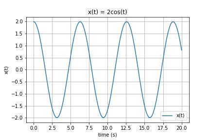
Would you look at that! The imaginary term disapeared, and finally we have a position equation thats a simple oscillator. You can do the same thing to figure out the equation for the velocity of the mass. Just plug in the constants $c_1, c_2$.

In summary, given a mass of $1$kg attached to a spring, with a spring coefficient $k = 1$, initial position and velocity of $x(0) = 2$ and $v(0) = 0$ its position is governed by the following equation:

$x(t) = 2cos(t)$

We can see this behaviour below in the position time graph. The mass oscillates forever since there is nothing to damp it's motion.

Method 4: Matrix Representation

Ok so we have a way to solve ODEs in a couple ways now. But what happens when we want to solve a differential system with multiple variables and their derivaties? First I'll motivate a matrix representation for our problems and then we can solve a harder system using the matrix representation.

Let's look at this example for now:

$\ddot{x} + 3 \dot{x} + 2x = 0$

$x(0) = 2$

$\dot{x}(0) = -3$

Using our previous methods we can just guess the function for $x(t)$ for now and figure out what it's first and second derivatives are and then see if we can solve the system.

$x(t) = e^{\lambda t}$

$\dot{x}(t) = \lambda e^{\lambda t}$

$\ddot{x}(t) = \lambda^2 e^{\lambda t}$

Now we have a function for $x(t)$ but we don't know what our parameter $\lambda$ is. We can do some simple substitution into our system to try to figure out what $\lambda$ has to be.

$\ddot{x} + 3\dot{x} + 2x = 0$

$\lambda^2 e^{\lambda t} + 3\lambda e^{\lambda t} + 2 e^{\lambda t} = 0$

Factoring $e^{\lambda t}$ out we get:

$e^{\lambda t} (\lambda^2 + 3\lambda + 2) = 0$

This equation is true in two cases. The first, which is not that interesting is when $t = 0$. The second is when $\lambda^2 + 3\lambda + 2 = 0$.

Solving this using the quadratic formula we get the values of $\lambda = -1,-2$. As before, to get a general solution you would have to solve for $c_1$ and $c_2$ using the initial conditions provided:

$x(t) = c_1 e^{-t} + c_2 e^{-2t}$

I'll leave that to you as an exercise and instead we'll investigate an interesting idea. If you look closely at the equation we solved in terms of $\lambda$ it might look familiar from a linear algebra class. Perhaps because of the use of the variable $\lambda$ you might think this could be the characteristic polynomial of a matrix.

Another way to look at this system is as a set of two equations which we can turn into a linear system and then solve. Rearranging our linear ODE equation we get the following two equations.

$\dot{x} = v$

$\ddot{x} = \dot{v} = -3\dot{x} - 2x$

We can take the variable and it's first derivative and represent both of them at the same time as a stacked vector. We can then write our system as follows in the form $\dot{y} = Ay$:

$ \frac{d}{dt}\begin{bmatrix} x\\ v \end{bmatrix} = \begin{bmatrix} 0 & 1\\ -3 & -2 \end{bmatrix} \begin{bmatrix} x\\ v \end{bmatrix} $

You can verify that this represents our system faithfully. Now, let's try to figure out what the eigen values are for our matrix $A$. This is typically done by solving for $\lambda$ in the following equation:

$det(A - \lambda I) = 0$

$det[ \begin{bmatrix} 0 & 1\\ -3 & -2 \end{bmatrix} - \lambda I_2] = 0$

$det[ \begin{bmatrix} -\lambda & 1\\ -3 & -2 - \lambda \end{bmatrix} ] = 0$

$(-\lambda)(-2-\lambda) - (-3)(1) = 0$

$\lambda^2 + 2\lambda + 3 = 0$

This yeilds the characteristic function for the matrix $A$ which interesting also happens to equation we solved previously for $\lambda$. This isn't a coincidence!

---

Higher order linear systems

• Introduce matrix representation
• Show solution for decoupled system
• Show relatedness of general ODE system to its matrix representation
• Introduce eigen decomposition
• Show solution to general linear system problem

Discrete Solutions

• Show different types of integrators: Forward Euler, Backward Euler, RK2, RK4, Symplectic Euler
• Analyze global and local errors of methods
• Show some real world examples